The farmers with the least land, the least capital buffer, and often the least physical capacity to adapt quickly are disproportionately the ones farming in Taiwan’s most volatile microclimates.
Several of the counties with the oldest farming populations are also seeing among the sharpest rises in heat stress. Since 99% of Taiwanese farmers work under 2 hectares, individual ownership is arithmetically out of reach for nearly the entire target sector. Soil classification accuracy doesn't just affect the map; it determines whether the ownership model above is financially viable in a given township. This is the strongest argument for replacing the placeholder classification with parcel-resolved TARI soil survey data.
Precision agriculture offers compelling logic, but it was built for scale — capital, infrastructure, and land large enough to justify the cost. For Taiwan, an island committed to agricultural self-reliance, that model is the wrong shape. ReLEAF was built to reshape it.
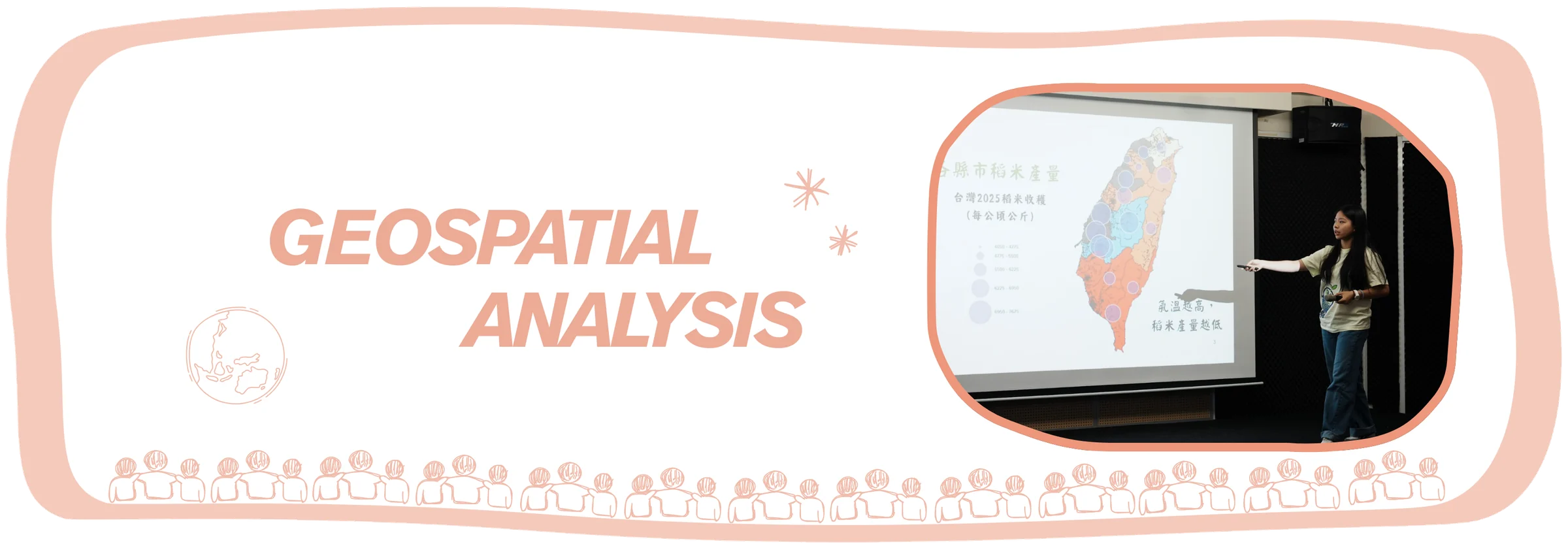
In Taiwan, 99.2% of farms are small-scale (under 2 hectares), yet together they work 85.3% of the island's farmed land, on terrain where a single region can span a temperature range rivaling the distance between Miami and Anchorage. This analysis uses geographic information systems to map where that mismatch becomes measurable: where accelerating warming converges with the farmland smallest in scale, oldest in stewardship, and least resourced to respond, and where centralized solutions like protectant distribution add distance and cost rather than closing the gap and addressing the need. Farmer interviews and field visits across farmers’ associations confirmed socio-scientific data patterns in lived experience.
This convergence of stress, vulnerability, and infrastructural mismatch is what ReLEAF answers – a decentralized biomanufacturing system built to put precision-level responsiveness directly into the hands of individual smallholder farmers, at a scale precision agriculture has not yet been designed to reach.
Introduction
Single interviews cannot establish whether what one farmer describes is an isolated hardship or a structural pattern. Answering this requires working at a different scale entirely: parcel-level land records, station-level climate data, and demographic surveys, aggregated across all counties rather than gathered farm by farm. This is where the role of geospatial analysis comes in, complementary to case studies.
Existing geospatial studies of Taiwanese agriculture tend to treat variables in isolation: climate-trend analyses map warming or rainfall change without reference to who farms the affected land, while agricultural demographic surveys report vulnerability without a spatial climate layer to test it against. None, to our knowledge, overlay farmland fragmentation, climate volatility, and a documented crop-stress yield effect at the parcel or township level simultaneously. This page explains our journey and findings in doing so.
Beyond layering maps, geospatial analysis feeds the math model’s simulations for the business plan; it is checked against wet lab's own stress-response data, so the map's "who needs this" and the bench's "does this work" can answer each other; and it's cross-referenced against Human Practices' direct farmer interviews, so the pattern in the data is tested against what people are actually living through.
Problem statement
Global climate stress
Rice is the primary calorie source for more than half the world's population, and across Asia it is grown at every scale — from smallholder plots to industrial acreage — as both a staple food and an economic backbone. The most dangerous part of this dependency is not the stress a farmer can see coming; it is the stress that arrives when no one is in the field to see it—during night time.
Farming has always been a practice of response: a farmer notices wilting, discoloration, or dry soil, and intervenes. That model assumes stress leaves a visible trace in time to act on. Rising nighttime temperatures break that assumption. A 25-year record from the International Rice Research Institute’s farm in the Philippines (Peng et al., 2004) showed that from 1979 to 2003, nighttime minimum temperatures rose roughly three times faster than daytime maximums, and that dry-season grain yield fell by about 10% for every 1°C rise in nighttime temperature, while daytime heat alone had no significant effect. The leading explanation is that warm nights keep the plant’s metabolism running in the dark, burning through the sugars it stored during the day before they can be committed to grain.
What matters most here is not the size of that loss but its timing. The damage happens overnight, leaves the canopy looking entirely healthy by sunrise, and only becomes visible weeks later as a lighter harvest. A run of warm nights during grain filling can cost a season’s yield one year and miss the critical window entirely the next, so there is no reliable signal to watch for and no point at which a farmer could have stepped in. Even an attentive, experienced farmer cannot respond to stress that happens on the plant’s schedule rather than their own. As warming makes these events more frequent and less predictable, protection that waits for symptoms will increasingly arrive too late.
Figure 1Global rice Yield Documentation to Forecasting: Year 2006 to 2100
Referring to Figure 1, the global yield projection shows the scale of what is at stake: much of the world’s high-yield rice belt sits inside a temperature band that is now shifting. Zoomed out, this looks like a distant problem. Zoomed into any single country with a rice-dependent food system, the problem is urgent — and Taiwan is one of the clearest cases of that shift already underway.
Revealing climate stress and farmland
Taiwan’s geographical and climate variability arguably makes the island’s farmers more vulnerable to agricultural stress. Taiwan is barely 400 kilometers long, yet it holds both a tropical and a subtropical climate. A three-hour drive crosses a temperature range of roughly 19ºC.
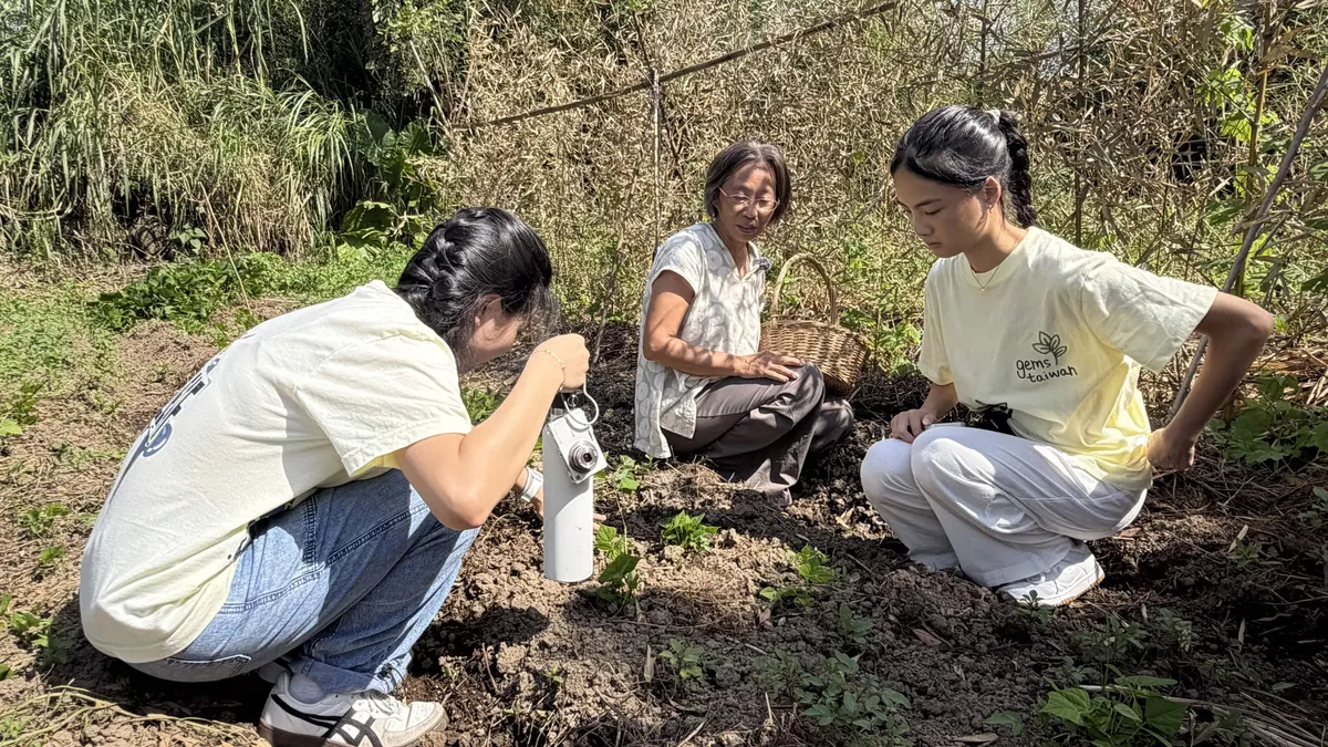
This compression extends underground as well. Ms. Chen, who has run a natural farm in northwest Taiwan for 25 years, put it simply in our field visit:
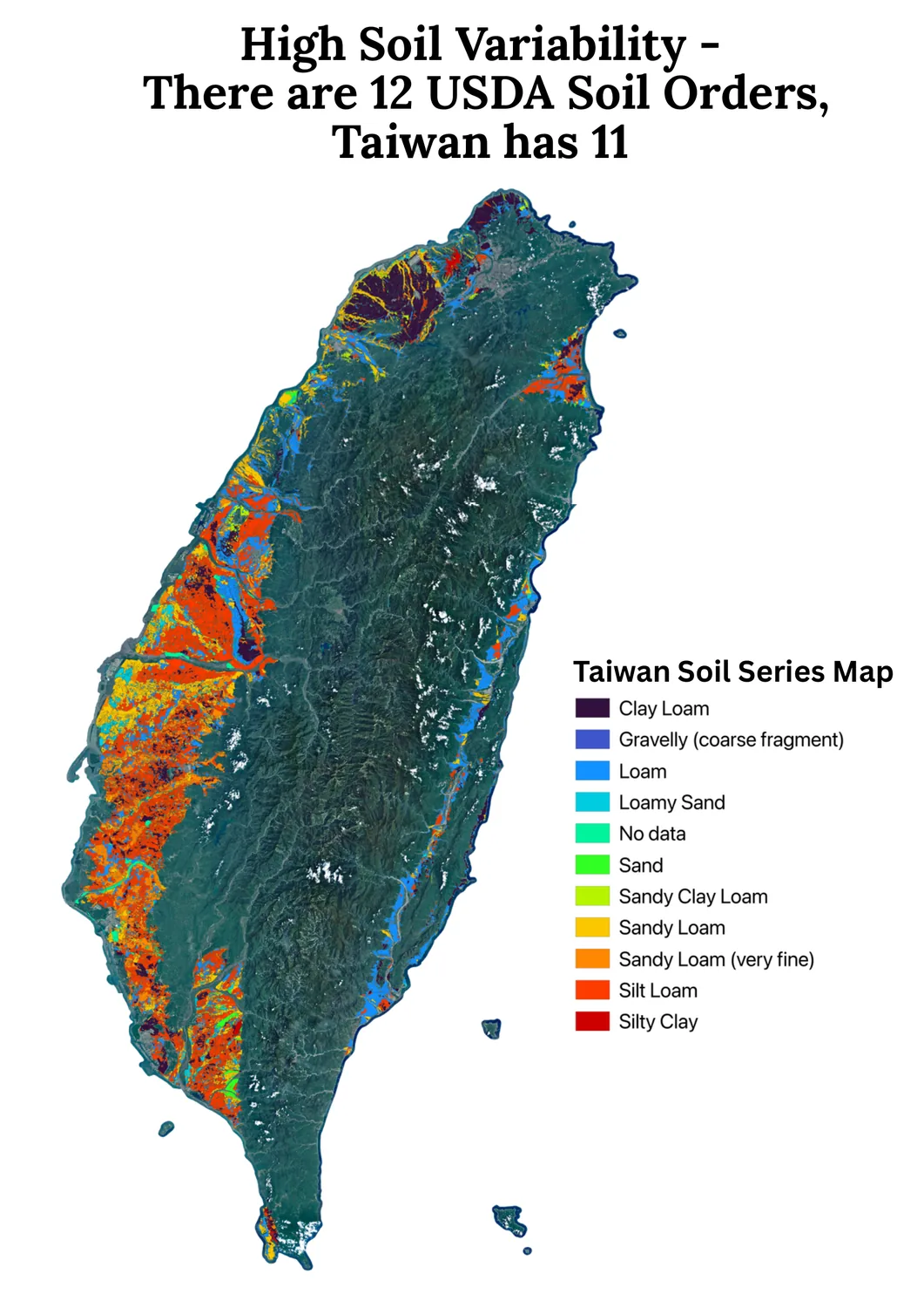
“Even the world’s top soil microbiology PhD doesn’t fully understand Taiwan’s soil… Earth has about 12 soil classification types, and Taiwan alone has 11 of them.”
All variability stacked together, rather than one broad agricultural tradition, Taiwan’s farming knowledge has evolved into thousands of hyper-local, inherited practices, each tuned to a single slope or valley.
Figure 2Soil variability.
Figure 2 is the visual argument behind Ms. Chen’s quote: soil shifts, soil type shifts block by block along the western plain, from alluvium to schist to mudstone. Thus, being in the same county doesn’t assure similar planting methods. Consequently, a farming method tuned for one farmer can be the wrong answer for another.
The underlying fragmentation innate to Taiwan is now colliding with a warming rate that continues to outpace tradition’s ability to adapt. For nearly a century, Taiwan’s average temperature crept upward by around 0.11ºC per decade – slow enough that a farmer could spend a lifetime farming and barely notice. Since 1991, that rate has nearly tripled to 0.29ºC per decade, with 2024 becoming Taiwan’s hottest year on record, with Taipei logging 63 days above 35ºC. Refer to Figure 3 for visualized crop yield changes in response to increasing heat stress.
When asked how she prepares for the dry season, Ms. Chen described layering dried weeds across her soil so morning dew soaked slowly into the ground, carrying her plants up to three weeks between checks. It is a schedule calibrated over decades on one plot of land, and it assumes stress will build at the pace it always has. Contrary to the certainty, a 2022 global study led by Hong Kong Polytechnic University found roughly 34-46% of flash droughts reached drought conditions within five days, with that share rising over 2000–2020 while frequency mostly held steady. Farmers’ knowledge hasn’t changed, but the window it was built for has shrunk. Closing that gap means protection already in place before stress arrives.
Taiwan agricultural demographics
In Taiwan, 99.2% of farmers are small-scale farmers (< 2 hectares of land). Their average farm holds just 0.9 to 1.1 hectares. Yet, together, small-scale farmers hold up to 85.3% of Taiwan’s arable land.
The average Taiwanese farmer is 63.5 years old, and more than half of all farmers are over 65. Accurate, early response to crop stress has traditionally depended on someone who can walk a field and read it; yet, that skill is disappearing as the farming population ages.
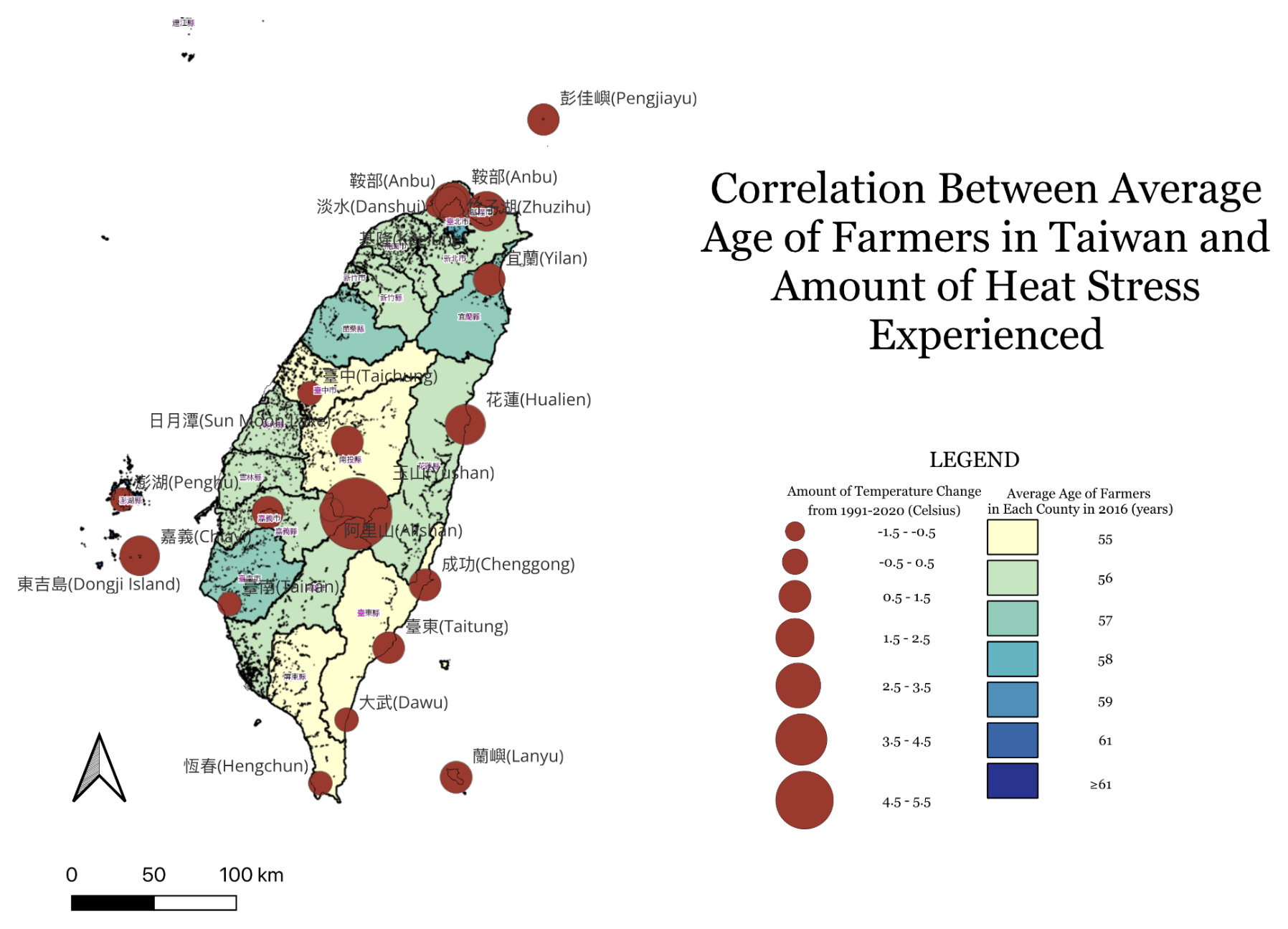
Overlaying county-level farmer age against temperature change from 1999 to 2020 (refer to Figure 4) shows these two burdens are not independent: several of the counties with the oldest farming populations are also seeing among the sharpest rises in heat stress. This means the demographic least equipped to respond quickly is concentrated in the places where conditions are changing fastest.
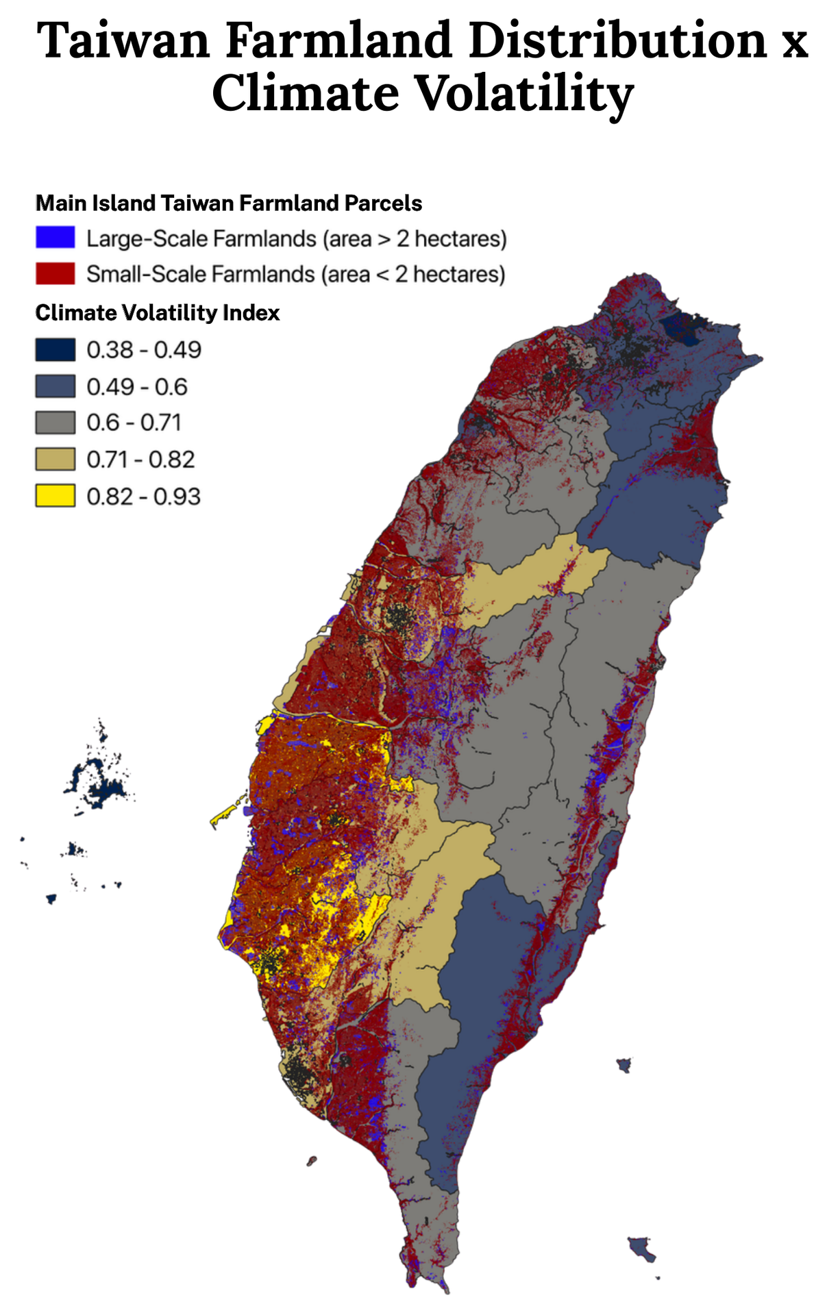
Figure 4Average Age of Farmers vs. Heat Stress Intensity.Figure 5Taiwan Parcel Farmlands x Climate Volatility.
Figure 5 shapes the picture further. Small-scale farmland (red, under 2 hectares) clusters heavily along the western plain and southern regions – the same areas that overlap with higher climate volatility index bands (computed through mean diurnal temperature range, seasonal temperature range, precipitation coefficient of variation, etc.). The farmers with the least land, the least capital buffer, and often the least physical capacity to adapt quickly happen to be the ones farming in Taiwan’s most volatile microclimates.
Centralized vs. decentralized agriculture
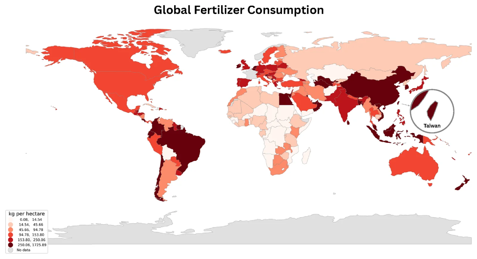
Taiwan, at just 36,200 square kilometers, consumes more than 300 kilograms of fertilizer per hectare – compared to roughly 128 kilograms per hectare in the United States, a country 9.83 million square kilometers in size (Refer to Figure 6 and Figure 7). Part of this gap comes down to spatial pressure: only about a quarter of Taiwan’s land is viable for agriculture, versus roughly two-fifths in the US. But fertilizer use scaled to compensate for land scarcity comes at a cost. While fertilizer has propped up yields, excessive application strains underground soil biology and degrades soil quality over time.
With the socio-geographic combinations of Taiwan demonstrated through visualized location-based data, there is a mismatch. A blanket fertilizer strategy is, by definition, poorly matched to a landscape this fragmented—a prominent example being Taiwan—it overcorrects in some regions and undershoots in others, because it was never built to respond to hyper-local variation in the first place.
Figure 6Global Comparative Fertilizer Consumption (Unit: Kilograms per Hectare).
That centralization problem isn't just chemical — it's logistical. To quantify it, we built a nationwide GIS routing model connecting every one of Taiwan's 613 registered fertilizer companies to real farmland (Refer to Figure 8): 2,792,536 individual parcels, aggregated by township into 346 demand nodes covering roughly 743,500 hectares of arable land. Each company is routed only to farmland inside its own county, using live road-network distance rather than straight-line distance — the model won't let a company shortcut to a closer field across a county line, because that's not how actual distribution works.
Figure 8Fertilizer and Agrochemical Footprint from Corporation to Farms. Open it full screen
Even under this best-case, same-county assumption, the model shows that centralized fertilizer production still has to travel: every kilogram makes a real trip along real roads before it reaches a real field, adding cost for cold chain, time, and emissions that a farm averaging under 1.1 hectares absorbs disproportionately relative to its output. A production model that instead manufactures the protectant on-site — at the scale of a single farm or a shared township reactor — removes that shipping step entirely. There's no freight distance to close, because there's no freight.
Through the tool of Geographic Information Systems and conversations with farmers, we understood closely that farmers have persevered so far by drawing on generations of accumulated, hyper-local expertise. But climate unpredictability has opened a gap between how fast that tradition can adapt and how fast the climate is now changing — and centralized, one-size-fits-all interventions, whether chemical or logistical, aren't built to close it.
Execution
Execution: GIS and Wet Lab
By incorporating GIS into ReLEAF—from LPA measurement and plant assays—the team is able to analyze lab-scale efficacy test results to quantify and predict real-field spatial deployment.
In consideration to confirming and quantitatively measuring on-site on-demand deployment in fields, a highly important factor to consider is how well our engineered bacteria responds to light, how quickly is the response, and how much protectant is ultimately produced. The Light Physical Activity (LPA) allows for quantitative analysis and accurate measurement rather than blindly answering these concerns qualitatively.
The LPA is a 24-tube LED array that holds engineered B. subtilis WB800 (CcaS/CcaR system) under six defined light conditions at once: green light (~535 nm) induces protectant production, and red light (~670 nm) halts it. Each condition is one column of four resistance-matched LEDs lighting four tubes. Intensity is set by Arduino PWM through three MOSFETs, one per tier (low, mid, high), and held constant for the whole run. Rather than a single endpoint reading, we sample each condition over time and track protectant output across the full period.
What we are measuring:
Production Timeline
How long after induction the protectant becomes detectable, and how that timing shifts with light intensity (low, mid, high) and wavelength (green vs. red).
Total Yield
This depicts how much protectant a culture is able to produce under a given light threshold, the following allows for a direct comparison of the yields across varying light intensity conditions.
The LED characterisation, build details, and results as they become available are documented on the LPA hardware page.
Contribution to the math model
The production rate from the LPA is a direct input to Stage 2 of the Math Modeling sector (DryLab × GIS). There, it converts specific enzyme activities into a volumetric production rate. That rate is what the model needs to calculate coverage radius, deployment density, and units per hectare. Production rate depends on the light regimen, so it is carried into the model as a range across conditions rather than a single value. This ties the light each unit receives in the field to how much protectant it delivers per hectare.
Confirming the efficacy of ACCD is not equivalent nor similar to confirming that ACCD has reached the plant. The project is deemed useless if the protectant never reaches the root zone. Functional Assay Validations account for this flaw, it measures whether treated plants actually perform better under stress than untreated ones, using physiological readouts rather than assumptions. By evaluating these factors functional assay validation runs in four linked stages, each stage's output narrowing the confidence with which ACCD efficacy data can be used elsewhere in the pipeline:
Physiological readout selection — chlorophyll a+b content as a quantifiable proxy for salt-stress damage
Timing conditions — testing protectant delivery before, during, and after stress onset
Salinity gradient — testing across 0, 75, and 100 mM NaCl to capture dose-dependent response
Cross-system validation — repeating the same assay across agar, hydroponics, and soil to test whether efficacy holds as the growth environment moves from idealized to field-realistic
Chlorophyll content as a physiological readout
Chlorophyll degradation is one of the earliest and most reliable indicators of salt stress in plants. Sodium accumulation disrupts chloroplast structure, accelerates chlorophyll breakdown, and suppresses photosynthetic capacity well before visible wilting occurs. Thus, chlorophyll content serves as a quantitative proxy for stress damage, and by extension, for protectant efficacy. A plant that retains more chlorophyll under identical salt exposure is a plant that is better protected.
We quantified chlorophyll a+b content spectrophotometrically, using absorbance readings at 645 nm and 663 nm following extraction in 80% acetone. Chlorophyll a+b content was quantified spectrophotometrically (OD645, OD663) following extraction in 80% acetone, using the standard formula
Meanwhile the results were reported both as raw concentration and normalized against fresh tissue weight. The two factors were both recorded to avoid misinterpreting the result.
Results
Untreated controls showed low chlorophyll content across all salinity levels, which suggests baseline chlorophyll extraction or growth conditions in this experiment were conservative rather than optimal, a detail worth accounting for when comparing absolute values across experiments. Every ACCD-treated group, regardless of timing, showed higher chlorophyll retention than its corresponding control at matched salinity.
Cross-system validation
Displayed in Table 1, the chlorophyll data above were collected on agar, including a controlled environment isolating ACCD’s biological effect on its transport variability. While agar does establish its existence and effect, it does not confirm its effect in real root-zone or external delivery.
System
What it tests
Validation Sector
Agar
Direct physiological effect, no transport confound
Baseline efficacy
Hydroponics
Liquid-phase delivery through root-zone water
Transport-dependent efficacy
Soil
Adsorption, degradation, heterogeneous flow through real soil matrix
Real-field testing
Figure 9Tested Systems for Arabidopsis and their purpose
From functional assay to GIS
Soil-validated efficacy data is what allows the five FVM soil-type coverage estimates covering the Math Modeling sector to be treated as measured results rather than untested projections. Without a plant-level confirmation that ACCD actually protects roots once delivered through soil rather than agar or liquid media, the coverage radius, deployment density, and unit-per-hectare figures downstream would all rest on a modeling assumption instead of a physiological result. This is the correlation between Wet Lab and GIS: the chlorophyll data is the evidence that the coverage radius GIS maps onto Taiwan's counties is protecting something real, something farmers can come to recognize as theirs.
Execution: GIS and Dry Lab
Next, utilizing geospatial analysis’ ability to link computations, simulations, and deployment plans to specific locations, we connected ReLEAF’s business plan and the math modeling powering it with GIS, using a calculator that computes the yield in which farmers are able to save alongside the implementation of our bioreactor.
The GIS page ends with a number: what percentage of farmers’ yield can we retrieve from the effect of heat and salinity stresses. Human Practices asks the four questions that decide whether that number ever becomes hardware standing in a field: is it legal, who holds the capital, what does it cost against what the crop is worth, and is it actually better than what the farmer does/ has today. Answering them requires two kinds of work in tandem: stakeholder engagement tells us what farmers, farmers' associations, and forum audiences will and won't accept, while desk analysis of Taiwan's statutes, farm economics, and the competing product landscape tells us what is permissible and affordable. Together they turn a deployment count into a deployable product.
Ownership model. Applying unit cost (US$937.50 per 20-litre unit, NT$30,000) to the deployment consideration: Since 99% of Taiwanese farmers work under 2 hectares, individual ownership is arithmetically out of reach for nearly the entire target sector. A shared-asset model through Taiwan's farmers' associations isn't a preference — it's the only ownership structure the numbers permit.
Organic regulation. Taiwan's Organic Agriculture Promotion Act excludes any product that is genetically modified from certified organic production, regardless of containment. Since ACC deaminase is produced by an engineered strain, this excludes ReLEAF from organic and friendly-environment farming; as about 3.7% of cultivated land, yet still a significant one, since these are the fastest-growing segments in Taiwanese agriculture and the audience most predisposed to adopt a biological input.
Cost. Depicted under the shared-ownership model, the number that is the most significant to a farmer isn’t necessarily the capital cost; rather the cost per hectare per season. This figure depends on the refill cartridge cost and hardware service life, while the rice-straw-return mechanism provides an incentive for farmers to use our product, as they are able to exchange straw waste for reduced-price protectant, lowering cost without a subsidy.
Carbon footprint. Compared to decentralized fertilizers and market protectants, our on-site production removes the emissions tied to industrial synthesis, packaging, and shipping, and in return, introduces the drive of continuous electricity and hardware emissions instead. Although the decentralization isn't automatically lower carbon, as it depends on the cycle; a unit that only activates on a predicted or detected stress event is more effective than running continuously, making the agronomically precise deployment favorable.
Competitive position. Different from centralized biostimulants and live engineered microbial inoculants, ReLEAF’s bioreactor presents a distinct position as it is delivering an engineered biological function to the plant without releasing the engineered organism into the environment, all alongside remaining adjustable based on the different crops. Despite these benefits, the product still poses as a competitive risk as it may be a relatively more rational choice for a farmer under seasonal cash constraints with doubt towards a newly presented project to choose an on-the-shelf product.
Back to GIS
Derived from the math modeling indications, the soil type with the highest volatility is sandy loam, while it also is the coastal soil class this project's current geomorphology-based classification heuristic assigns most broadly. That means that the soil classification accuracy not only affects the map but also determines whether the ownership model above is financially viable in a given township.
Validation
Problem validation
Through a public forum held with farmers across agricultural regions in Taiwan, namely Nantou, Hualien, Hsinchu, Yilan, etc., we collected interview data from farmers planting various plants—like cocoa, rice, coffee beans, and mixed grains. Spanning across crops and farm scales, we identified a consistent pattern that has emerged within the last 5 years: soil management is conducted based on habit, as they perceive it as extra money spent on seemingly useless data.
“Not directly, farmers do not manage it [soil]”
Cocoa Farmer from Nantou
This statement demonstrates the evident validation of IHP, establishing the gap coverage that the problems identified are not limited to rice cultivation, but relevant to all smallholder agriculture in Taiwan, relating to soil management.
Inconsistent soil testing
After visiting numerous booths, most of the interviewed farmers applied organic fertilizers based on a fixed annual schedule, not based on current soil deficiencies or environmental changes. At farms where soil testing does occur, it has a tendency to be limited in frequency: a mixed grain farmer receives one free test from the government per year, and so do farmers in Miaoli; while they stated, in addition to the free one, they wouldn’t go out of their way and pay more for calculated numerics. Meanwhile, the cocoa farmer quoted above consults no expert whatsoever.
Contrastingly, there are notable exceptions, as different farmers with varying crops tend to have different perspectives and priorities in order to maximise their yield, and what they value: money, yield, the joy of it. For example, on the contradictory to people who don’t test, pear and peach growers from Hualien mandates soil testing and treats calcium deficiency as disqualifying for certification, while a persimmon farmer in Hsinchu independently targets a substrate pH of 5.6 to 6.2, having begun from an initial pH of 3. These two cases demonstrate that data-driven soil correction is effective when implemented, but they also represent exceptions rather than common practice. This finding indicates a gap that a passively deployed bioreactor is designed to address, as it delivers a corrective response without requiring the farmer to first acquire diagnostic capability that most currently lack and do not actively pursue.
The Nantou farmer’s response to any proposed treatment was specific and immediate: a natural protectant would be acceptable, provided its compatibility with organic certification requirements could be confirmed. This farm is in the process of transitioning to certified organic status, and any input under consideration must remain compatible with that transition. This has direct implications for product positioning: a biological, non-synthetic treatment such as ACC-deaminase PGPR is not merely acceptable to this segment of farmers but may represent the only category of input such farmers are willing to consider. This also identifies a concrete requirement for market entry, as confirming compatibility with organic certification standards is not a clean line, rather a grey area, making farmers in their trial stage of the organic transition unwilling to risk it and try out the product.
Growing economic conditions motivate adoption and inheriting farms
Documented within Table 2, numerous farming locations have already exceeded the optimal temperature for plants to survive. Throughout the conversation with a Nantou farmer, they present a clear illustration and will to turn small farming into a business as time progresses. He expresses that the farm was originally cultivated solely to supply food to the farmer's family, with no intent towards expansion. This was until the responsibility of maintaining the growing land of previously owned aging parents, combined with the increasing food demand, prompted their agriculture to shift towards commercial production. They’ve established that the agricultural labor force is aging, as profit margins remain narrow with pest control left unattained, and the farmers are nonetheless actively working to establish a product following organic regulations. This represents the customer profile most relevant to IHP: small-scale farmers seeking to optimize profits while reducing manual labor.
Farmer’s Main Crop
Farmer Location
Farmer Location’s Average Temperature (ºC)
Cacao
Nantou
24.3
Peaches and Pears
Hualien Zhonghe
24.2
Cacao
Pingtung
25.9
Coffee Beans
Guanxi Mawudu
24.5
Fruit Trees
Xingzhu
24
Rice and Fruits
Yilan
23.4
Mixed Grains
Chiayi
24.3
Fruit Trees
Miaoli
23.3
Vegetables
Hsinzhu
24.5
Fruits & Vegetable
Yilan and Taichung
23.4 & 24.5
Figure 10The average temperature of the Farm location relative to the crop harvested.
Impact: current reach and future prospect
Considering that we want to choose a more vulnerable and high economical value crop so that we can sell more bioreactors and generate more profit, we looked into crops outside of rice. That led us to tomatoes - breeds like Beef Tomatoes can sell for all the way up to $201NTD per kilogram, and averages 152.9 per kilogram, making it a very high value crop (Taiwan Ministry of Agriculture 26).
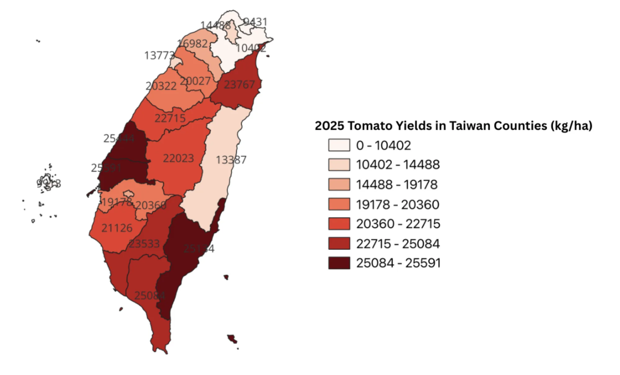
Taiwan’s tomato industry covers over 4,000 hectares of farmland in Taiwan and is concentrated within a few counties. According to the Agricultural Knowledge Retrieval Platform, farmers harvested across 3,627.94 hectares, yielding approximately 83.27 million kilograms in total, averaging 22,953 kg per hectare. Chiayi alone planted on 830.68 hectares of land and produced over 17.18 million kg, followed by Yunlin County, which produced 12.24 million kg; Kaohsiung City with 11.36 million kg, and Tainan City with 10.06 million kg (Refer to Figure 11).
Figure 11Tomato Yield per Hectare by County, Taiwan, 2025.
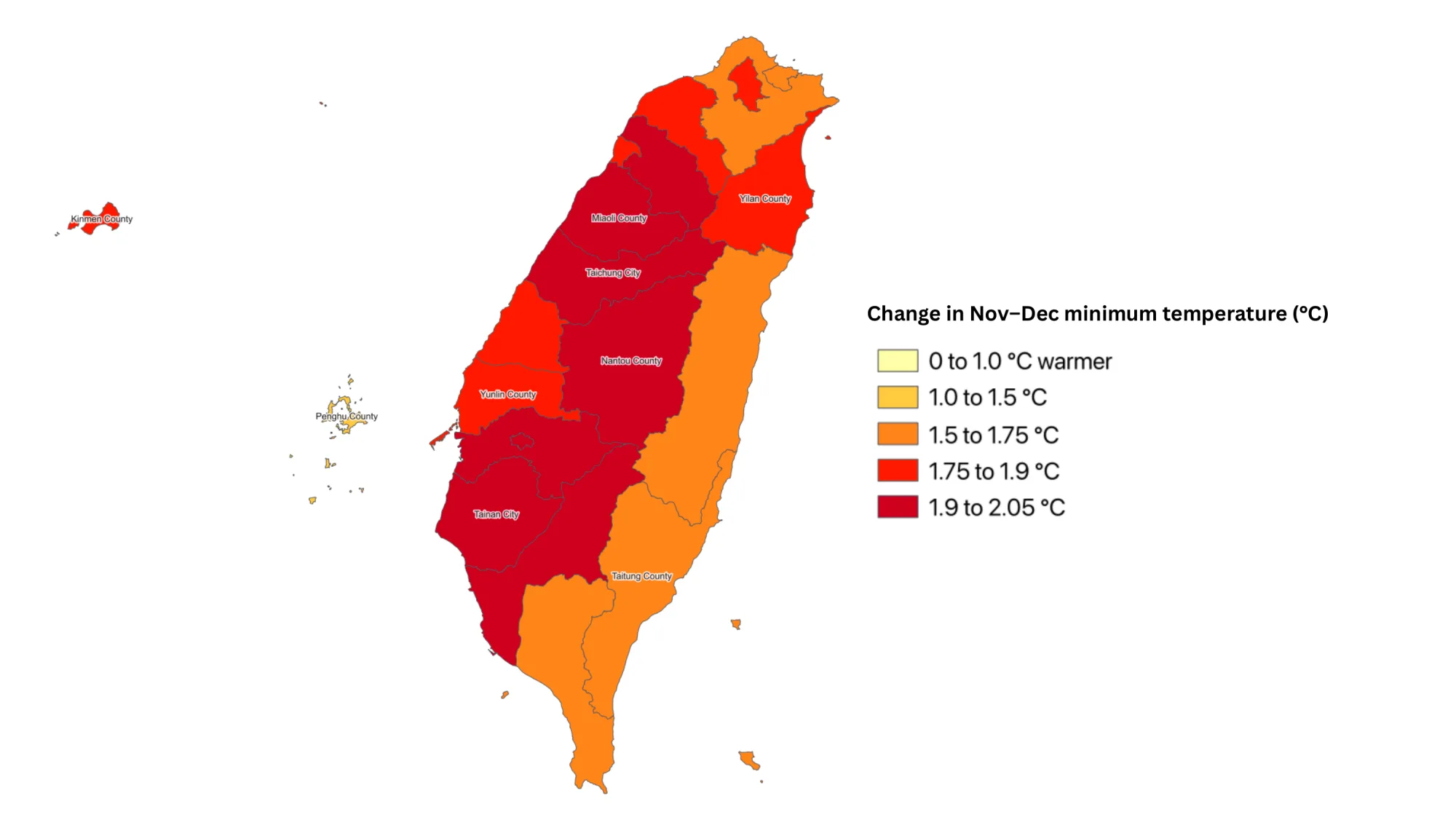
As demonstrated through Figure 12, the amount of increase in average November–December lowest nighttime temperatures in each county between 1961–1990 and 2015–2024, using ERA5 reanalysis data. November and December are when Taiwan’s main tomato crops flower and grow fruit, and they need cool nights. Every county warmed by between 0.9 °C and 2.0 °C. The largest increase, 1.9–2.0 °C, runs down the west-central spine of the island from Miaoli through Taichung and Nantou to Chiayi, Tainan and Kaohsiung. Together with Yunlin and Changhua, these counties grow 85% of Taiwan’s tomatoes. The east coast and the north warmed less, and Penghu the least, because the surrounding sea buffers night temperatures.
Figure 12Night-Time Warming During Tomato Flowering, 1961–1990 to 2015–2024.
Understanding the impact of recent fluctuations in climate on tomato yields shows that the crop can potentially be one of the crops that we target for the business plan, as the map proves that temperature has increased drastically in recent years, which makes it so that Taiwan’s tomatoes have become one of the crops that are most susceptible to heat stress. While rice is still a crop that’s susceptible to heat stress, tomatoes present a more viable option, as Taiwan is actually currently overproducing rice. That was confirmed by Director Wu, Tzu-Hsien, compounded by the fact that she also stated that tomatoes are also one of the most economically valuable crops in Taiwan, which means that tomato farmers will also be more willing to spend money to maintain and protect the quality of their crops. Through this, we can conclude that tomato farmers are a better target demographic than rice farmers in Taiwan.
Figure 13Farm Calculator: What ReLEAF Means For Your Field. Open it full screen
Contribution and tools
Guide
This guide is for teams new to GIS, as this tutorial covers 2 core fundamentals; switching between raster and vector data, and how to import data through three main data formats commonly accepted by GIS: GeoJSON, CSV, and Shapefiles (.shp). If the researched data sets are not in these three formats (eg., tables) or contain variances among the data (eg., different coordinate systems, unwanted data), you can reference the LLM broad prompt below, providing high efficiency when dealing with these issues.
To allow non-professionals or people interested in utilizing geospatial analysis/ GIS in their projects, we put together a practical guide covering how to distinguish and navigate through raster vs. vector data; additionally, how to import the three files into the aforementioned formats.
Rasters vs. vectors
As previously mentioned, Raster data and vector data are the most common and fundamental data types utilized within QGIS, one covering pixels, and the other utilizing lines/ points. Raster data sets are discrete and continuous cells (pixels) that represent data that gradually varies across space, also classifying them into different categories. Oftentimes, Raster data is used to present temperature or elevation maps as they can be visualized as continuous and gradient-like. Conversely, Vector data are scalable values that only depict discrete features like data points or lines; they are most commonly used to establish borders or outlines of files.
Importing CSV files
CSVs are the most common way to present data (eg., farm locations, sensor readings)
Has to include longitude and latitude within the 2 separate columns
Can only be imported to GIS through delimited text file
Unable to be picked directly from the browser window
Make sure to clearly define the Coordinate Reference System (CRS)
(eg., EPSG:4326 / WGS 84)
Importing GeoJSON
GeoJSON is a readable format for vector types, commonly found for web-based mapping
Import directly via Layer → Add Layer → Add Vector Layer, or by dragging the file into the Layers panel.
GeoJSON typically embeds its CRS in the file itself, but confirm it matches your project CRS before combining it with other layers
Mismatches here cause layers to silently misalign rather than error out.
Importing shapefiles (.shp)
Shapefiles are the standard vector format
Can be easily imported by finding the file within the Browser tab, and dragging the following onto the Layers tab.
LLM broad prompt
When researching global geospatial data, running into data sets with hundreds to thousands of numerics is inevitable. Oftentimes, these data sets are unorganized and condensed with tons of information often deemed too complicated for QGIS to directly utilize. Moreover with varying coordinate systems, data from different sources may have varying coordinates, unaligning in the software. Manually reconstructing thousands of numerics is time-consuming and could contain operator error, especially for students unfamiliar or non-professionals of the GIS field.
To address the following, we developed a broad, reusable prompt that generates data files in formats that QGIS is able to properly analyze (GeoJSON, CSV, SHP) from arbitrary raw input data. The following prompt, rather than being hard-wired to only analyze data sets beneficial to our project (Taiwan Farmland and Climate Volatility), the prompt is generalized so that any team desirable of use Geospatial Analyses can adapt it to develop their own geographic data set.
We designed the following prompt as a contribution other future iGEM teams can utilize and incorporate into their own project. As aforementioned, when integrating spatial analysis into desired projects, regardless of the specific data sets, it is bound to run into similar data overload problems, utilizing this prompt allows for easier data organization experiences.
The prompt mainly consists of the following components:
Takes numerous complicated or inconsistent data sets and formats them as GIS-readable data
Locates and extracts existing coordinate fields (latitude/longitude, X/Y, or combined location fields) from the raw data, even when inconsistently labeled
Detects or infers the coordinate reference system (CRS) of the source data and states it explicitly before proceeding
Standardizes the coordinate system to the convention required by the destination software (e.g., WGS84/EPSG:4326 for GeoJSON, valid geometry types, .prj requirements for shapefiles)
Outputs a clean CSV, SHP, or GeoJSON file with consistent columns, ready to import directly into GIS software (QGIS)
Rules that the prompt follows
Only utilizes data provided; extracting or reformatting an existing coordinate (splitting a combined field, converting units, reprojecting a stated CRS) is allowed, but it never invents, estimates, or geocodes a coordinate or value that isn't derivable from the file itself
If a coordinate's CRS is not stated and cannot be reasonably inferred, it says so explicitly and asks rather than defaulting to an assumption
If the data set contains empty or ambiguous data, it flags this explicitly rather than filling it in or leaving it silently blank
If fulfilling the author's request requires calculations (distance, filter, percentages), the logic is transparently shown, not just the final result
If a coordinate or value looks unusable (out of valid range, inconsistent format, mismatched CRS across records), it flags this before using it
The output format is exactly what the author requests (GeoJSON, SHP, CSV), with the CRS of the output stated explicitly
Our prompt, presented in Text 1, demonstrates that rules are grounded in established prompt engineering research rather than built ad hoc. Restricting the model to only use provided data reflects grounding research, shown to reduce hallucination (Addlesee, 2024). Flagging missing, ambiguous, or unusable values instead of guessing reflects calibration and abstention research, addressing a known tendency of LLMs to answer confidently rather than admit uncertainty. Requiring transparent calculation logic follows chain-of-thought prompting, shown to improve accuracy on multi-step tasks (Wei et al., 2022). Detecting and stating the coordinate reference system before use follows self-verification prompting, where an assumption is externalized so it can be checked rather than embedded silently in the output. Finally, requiring the output to exactly match the requested format (CSV, SHP, or GeoJSON) reflects structured output practices common to established frameworks such as CO-STAR and RTF, which produce more consistent, usable results than open-ended formatting instructions.
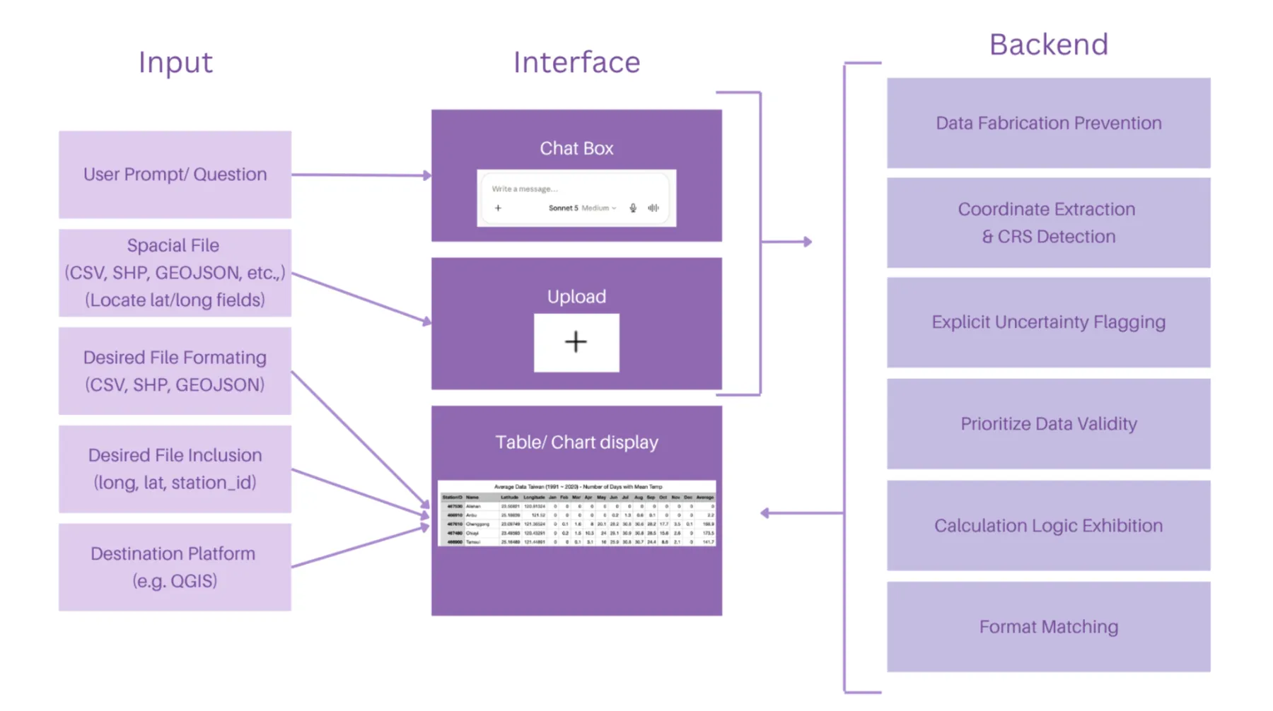
Depicted within Figure 10, the system architecture is organized into three interconnected layers: Input, Interface, and Backend, collectively supporting the operational deployment of the broad prompt.
Figure 14System Architecture and Implementation Layers of the Broad Prompt.
Text 1. Sample of the broad prompt
I'm working with spatial data that I need prepared for use in QGIS.

Current data format: [CSV / GeoJSON / Shapefile]
Desired fields in output: [e.g. site_id, latitude, longitude, organism, soil_type, ph, collection_date]
Desired output format: [CSV / GeoJSON / .shp]
Destination: This output will be loaded directly into QGIS for spatial analysis.
My question: [e.g. "convert this into a clean GeoJSON with only the fields I need"]

Step 1 — Locate the coordinates.
Before answering my question, find the fields in my data that represent location
(e.g. latitude/longitude, lat/lon, X/Y, easting/northing, or a combined
"coordinates" field). Tell me which columns you identified and what you believe
their coordinate reference system (CRS) is, based on the values and any metadata
in the file (e.g. values in the range -180 to 180 / -90 to 90 suggest WGS84;
large 6-7 digit values suggest a projected CRS like UTM). If the CRS is not
stated and cannot be reasonably inferred, say so explicitly and ask me rather
than assuming WGS84 by default.

Step 2 — Prepare for QGIS.
- Reproject/report coordinates so the final output is usable in QGIS. For
  GeoJSON, use WGS84 (EPSG:4326) with [longitude, latitude] order, per spec.
- If the source data is already in a projected CRS and I haven't asked for
  reprojection, keep the original values but state the CRS explicitly in your
  answer so it can be set correctly in QGIS.
- For shapefile output, note that a .prj file defining the CRS is required —
  tell me what it should contain.

Rules for your answer:
1. Only use values that are actually present in the file. Extracting or
   reformatting an existing coordinate (splitting a combined field, converting
   units, reprojecting a stated CRS) is allowed and expected. Inventing,
   estimating, or geocoding a coordinate that is not derivable from the file's
   own data is not allowed — flag those records as "missing coordinates" instead.
2. If a field is missing, empty, or ambiguous for a record, say so explicitly
   rather than guessing — flag it as "uncertain" rather than filling it in.
3. If my question requires a calculation (distance, area, count, filter), show
   your work or the logic you used, not just the final number.
4. If a coordinate or value looks unusable (out of valid range, inconsistent
   format, mismatched CRS across rows), point it out before using it.
5. Give me output in exactly the format I requested, ready to copy or download,
   and state the CRS of that output explicitly in your reply.
Validation
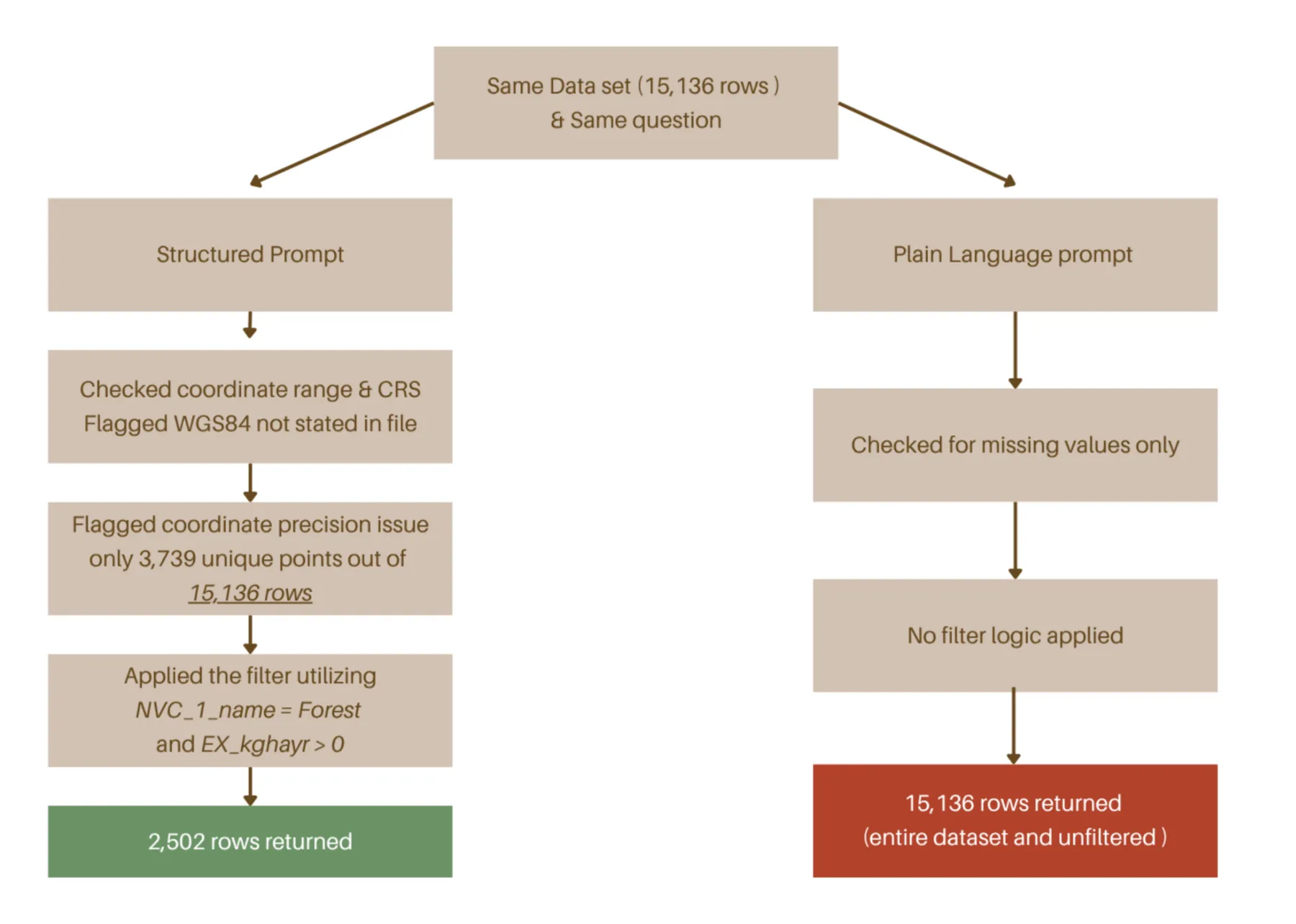
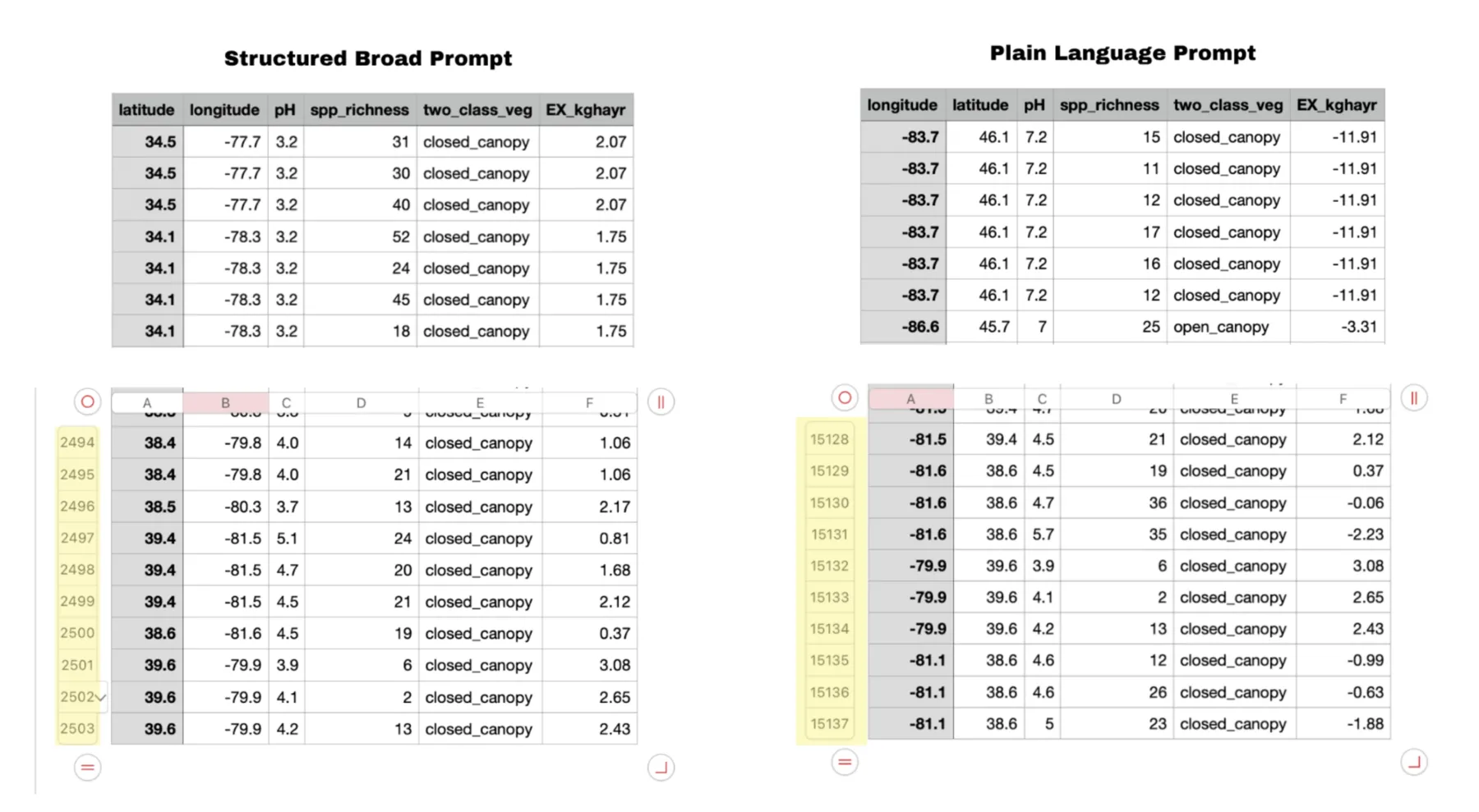
Figure 15Comparison Between the Structured Broad Prompt and the Plain Language Prompt.Figure 16Visual Demonstration of Prompt Efficiency Through Difference Between Number of Rows.
References
Central Weather Administration. (n.d.-a). CODiS climate observation data inquiry service [臺灣氣候觀測資料查詢服務; Data set]. Ministry of Transportation and Communications. Retrieved October 10, 2026, from https://codis.cwa.gov.tw
Central Weather Administration. (n.d.-b). 臺灣氣候 [Taiwan climate]. Ministry of Transportation and Communications. Retrieved October 10, 2026, from https://www.cwa.gov.tw
Chen, Li-Xing. (2026). 臺灣極端氣候對糧食作物的影響:以稻米、玉米及甘藷為例 [The impact of extreme climate on food crops in Taiwan: Rice, corn, and sweet potato] [Master's thesis, National Taiwan University]. NTU Theses and Dissertations Repository. https://doi.org/10.6342/NTU202601266
Ministry of Agriculture. (2024). Number of persons engaged in on-farm agricultural and livestock activities in agricultural and livestock households, by sex and age [Data set]. Taiwan Government Open Data Platform. https://data.gov.tw/dataset/80661
Ministry of Agriculture. (2025b). Taiwan's rice production per hectare for each county and city – rice (annual) [Data set]. Taiwan Government Open Data Platform. https://data.gov.tw/en/datasets/95738
Ministry of Agriculture. (2026a). Fertilizer management integrated information. Taiwan Government Open Data Platform. https://data.gov.tw/en/datasets/7304
農業部. (2026b). 臺灣地區肥料產銷量值 [Taiwan area fertilizer production and sales volume and value] [Data set]. 政府資料開放平臺. https://data.gov.tw/dataset/9690
Ministry of Environment. (n.d.). Taiwan soil information system. Environmental Management Administration. Retrieved September 26, 2026, from https://sqbs.moenv.gov.tw/public/English
Ministry of Environment. (2026). [Carbon footprint emission factors dataset (CFP_P_02)] [Data set]. Ministry of Environment Open Data Platform
Ministry of Transportation and Communications, Institute of Transportation. (2017). 公路貨運服務碳足跡公用係數建置計畫(2/2) [Establishment of general emission factors for carbon footprint of road freight transport services (2/2)]. https://www.iot.gov.tw/zh_tw/archive/pub/reports/-15034574
National Science and Technology Center for Disaster Reduction. (n.d.). 臺灣氣候變遷推估資訊與調適知識平台 [Taiwan Climate Change Projection Information and Adaptation Knowledge Platform]. Retrieved October 10, 2026, from https://tccip.ncdr.nat.gov.tw
Peng, S., Huang, J., Sheehy, J. E., Laza, R. C., Visperas, R. M., Zhong, X., Centeno, G. S., Khush, G. S., & Cassman, K. G. (2004). Rice yields decline with higher night temperature from global warming. Proceedings of the National Academy of Sciences, 101(27), 9971–9975. https://doi.org/10.1073/pnas.0403720101
QGIS Development Team. (2025). QGIS geographic information system (Version 3.44 LTR) [Computer software]. Open Source Geospatial Foundation. https://qgis.org
Qing, Y., Wang, S., Ancell, B. C., & Yang, Z.-L. (2022). Accelerating flash droughts induced by the joint influence of soil moisture depletion and atmospheric aridity. Nature Communications, 13, Article 1139. https://doi.org/10.1038/s41467-022-28752-4
World Bank. (2026). Fertilizer consumption (kilograms per hectare of arable land) [Data set]. World Development Indicators. Retrieved October 17, 2026, from https://data.worldbank.org/indicator/AG.CON.FERT.ZS