
Timing constraints on delivery
ReLEAF's reactor makes a protectant (throughout this page the protectant is modelled from our wet lab data on one of the protectants we engineered and produced, ACC deaminase) only while its green lamp is on, so the model has to set the light level and its duration. Sizing the system by volume, the litres of culture one hectare requires, gives an unstable answer, because that figure depends on a dose nobody has minimised and a canopy correction nobody has measured.
Timing is the better-posed problem, because three independent intervals have to fit inside one window. A weather forecast extends about three days. The reactor takes days to fill. The plant requires the protectant at a particular time relative to the stress, and that time is still contested at the bench.
The three intervals do not fit. One hectare's application takes 5.4 days on ten 20-litre units against a three-day forecast, so 2.4 days of production precede any forecast that would justify it. That is the co-treatment case, with the protectant arriving as the stress lands. If the agar result in M3 holds and the protectant has to be on the plant one day earlier, production starts 6.4 days ahead and 3.4 of those days precede the forecast. The reactor therefore cannot be scheduled from the forecast. It produces through the season and the forecast determines when stock is used, which makes the shelf life of that stock the controlling quantity on this page. M2 gives it a first value, indirect and unreplicated, and the value is short.
Model inputs and their provenance
Fourteen inputs feed this model: six are our own measurements, four are public records, two are published constants, one is a figure from Geospatial Analysis, and one is neither measured nor cited. That last is the canopy correction, a modelled term; the ledger in M4 shows where it enters and which rows inherit it. The final column of each table gives provenance, which sets how far a conclusion resting on that input can be taken.
Public record and literature
| Input | Source | What it sets | Provenance |
|---|---|---|---|
| County rice yields, every season since 2001 | Agriculture and Food Agency (農糧署) | Fits the stress index and scores it | public record |
| Daily weather, 2001 to 2025 | ERA5 reanalysis | The fifteen candidate stress terms | public record |
| Live forecast | Central Weather Administration (中央氣象署) | The three-day release decision | public record |
| Farm-gate paddy price, US$0.80/kg | Official 2026 farm-gate price | Turns an index level into money | public record |
| Unit cost, US$937.50 per 20-litre unit | Geospatial Analysis | Capital in the ledger | from GIS |
| CcaSR transfer function | Castillo-Hair et al. (2019) | The lamp setpoint; we have not tested it | literature |
| Enzyme kinetics, Km and kcat | Hontzeas et al. (2004) | Activity to protein mass | literature |
From our own bench
| Input | Source | What it sets | Provenance |
|---|---|---|---|
| Secreted activity, 7.25 mU mL⁻¹ | DNPH assay, 7 October 2026, n = 1 | Protectant per litre of culture | ours, below quantitation |
| Activity at 3 h and 6 h of induction | One tube at 3,850 lux, DNPH read at 28 h | The decay a banked stock has to survive | ours, n = 1 |
| Applied volume, 1.67 mL per three sprays | Experiment #9, phase 3 protocol | The dose, with the plate area | ours |
| Plate area, 78.5 cm² | 10 cm round plate, from the protocol | The dose, with the volume | ours |
| Timing arms, before / with / after | Three plant runs, two of them disagreeing | When the protectant must arrive | ours, contested |
| Reactor throughput, 34,807 mU L⁻¹ d⁻¹ | Titre over the batch cycle | Vessel litres per hectare | ours, derived |
| Rice canopy correction, ×2.44 | Leaf area index 4.5 against 0.115 on a plate | Plate rate to field rate | modelled, not measured |
Assumptions
Five steps in this model are assumed, not measured. Each is named below with the result that rests on it and the observation that would overturn it.
| Assumption | What rests on it | What would overturn it |
|---|---|---|
| A1. A yield below the county trend is weather damage | All of M1. The fifteen stress terms are fitted to that shortfall, so the county trend has to absorb variety change, mechanisation and management on its own. | A season whose shortfall came from pests, policy or a revised planted area; the index would read it as weather. |
| A2. The published CcaSR curve holds in a 20-litre vessel | The lamp setpoint, and Equations 1 and 2. The Hill parameters were fitted in small cultures under a light plate, and the same K1/2 and n are taken to hold at vessel scale and equal photon flux, with light reaching every cell alike. | An induction series at two or more intensities that does not follow the curve. Every run of ours was at one intensity. |
| A3. Dose scales with area, through one canopy correction | The whole ledger in M4. Millilitres per cm² on a 10 cm plate become litres per hectare through the factor C = 2.44 and nothing else, with spray interception, runoff and droplet coverage unchanged between a plate and a canopy. | Field spraying that leaves a different fraction of the applied volume on the leaf than a plate does. |
| A4. Secreted activity in the supernatant is the dose | The step from culture litres to protectant in M4, and the protein mass in Equations 3 and 4. The active ingredient is the secreted enzyme at its assayed activity, with Km and kcat from Pseudomonas putida UW4. | A contribution from the cells, the medium or a second secreted product, or activity lost between the assay tube and the leaf. The preparation sprayed on plants was never assayed. |
| A5. One pass protects for two days, and passes add up | The season in M5: nine passes, 49 reactor-days, 4.3% of the calendar and the capital per hectare that follows. | A protection window of any other length, or benefit that carries from one pass into the next. Nothing we have measured fixes the two days. |
Results
Stress index fitted to 25 years of harvests
Most crop stress indices weight temperature, water and light by expert judgement. Here the weights are fitted to Taiwan's harvest record instead. Taiwan grows two rice crops a year in the same field: the first crop (一期) is transplanted around February and harvested in June, the second crop (二期) in July and November. The two meet different weather, so they are fitted separately, and an index value is always quoted with its crop.
A season whose yield fell below its county trend was a stressed season. For each crop we fitted all 215 − 1 = 32,767 combinations of fifteen candidate stresses and scored every one on years it had not seen. The second crop pays for wind, light and badly timed water. Heat adds nothing once those three are included, which matters because the wet lab runs a heat programme this index does not support.
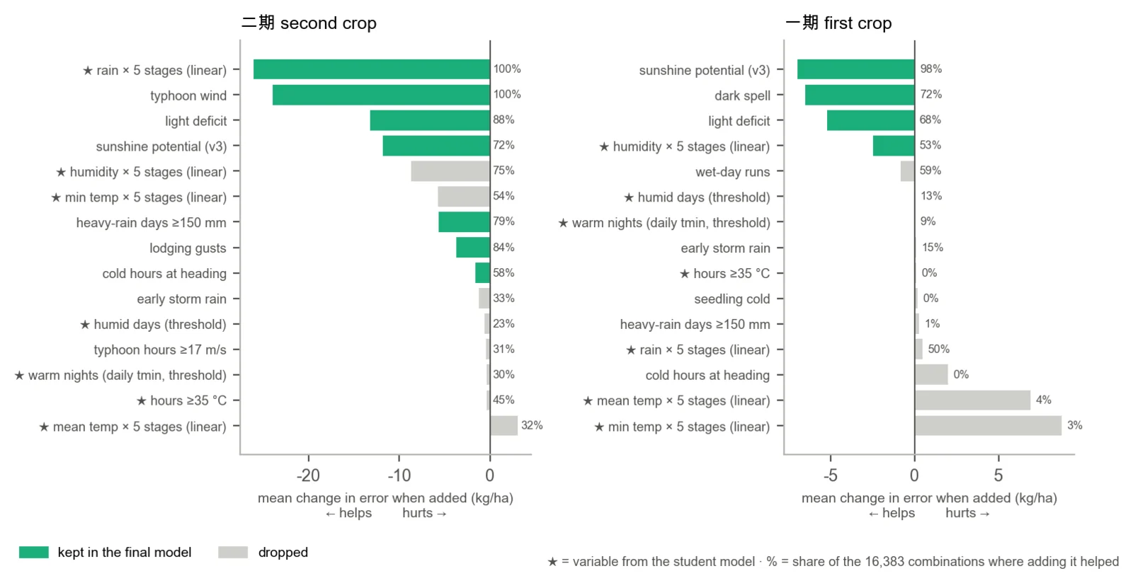
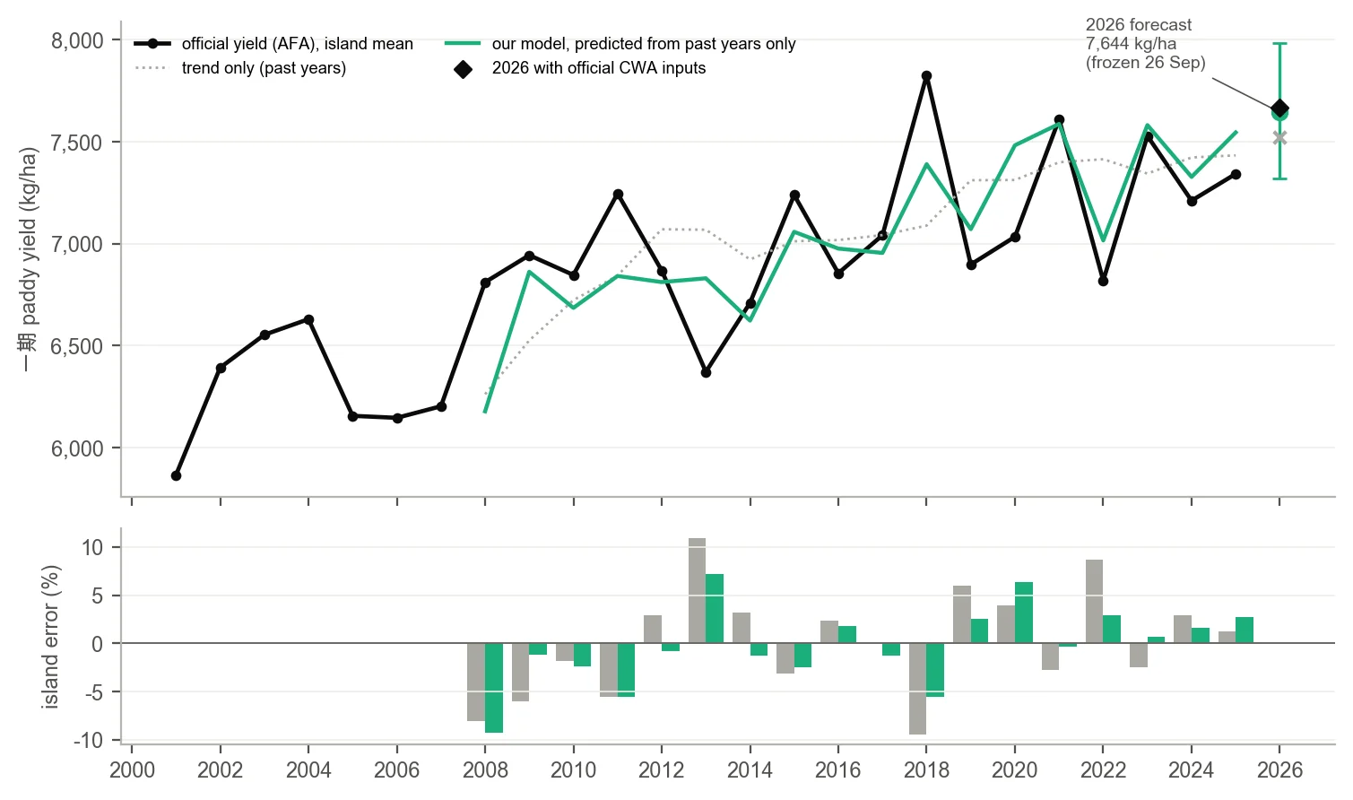
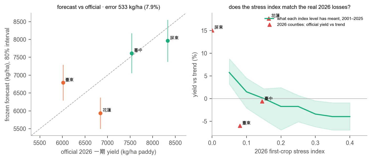
Against the no-weather trend the model carries 32% less county error in the second crop. The first crop is the weaker of the two fits and it is the one now being tested blind: the 2026 first-crop forecast was frozen on 26 September, before any county published, and four of sixteen counties have reported, at 7.9% county error against the trend's 8.8%. Four counties are too few to establish prospective performance. The model underpredicted Hualien and Pingtung and overpredicted Taitung; only Taichung fell close to its prediction. The second crop is not harvested until November, so the better-fitting of the two models has not yet been tested blind.
Induction at one intensity, and activity decay
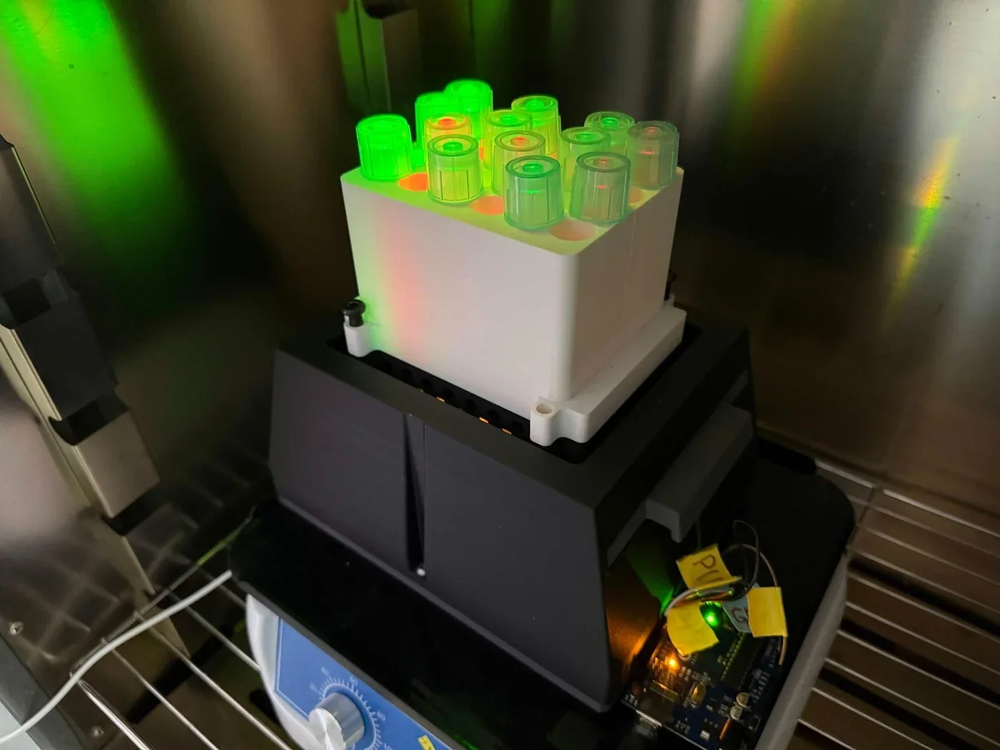
The reactor holds Bacillus subtilis WB800 carrying the cyanobacterial CcaSR system. Green light at 535 nm activates CcaS, CcaR~P drives PcpcG2, and the protectant gene behind a secretion signal puts active enzyme in the supernatant. The intensity that gives a target output comes from the Hill function Castillo-Hair et al. (2019) fitted in B. subtilis, inverted; both appear in the Equations section. We take that curve as published. Nothing we have run tests it, because every induction so far has been at one setting.

Measured activity at three and six hours
One tube was held at 3,850 lux of green and sampled twice, at three hours of induction and again at six. The assay signal did not accumulate between those samples. It fell, from 0.5503 mM of α-ketobutyrate to 0.1414, or 26% of the three-hour value. Read as first-order loss through two points, that is an apparent half-time of 1.5 hours.
Two limits apply to that figure. The tube was still producing enzyme across the interval, so the decline is a net quantity and the underlying decay is at least this fast. And the measurement is of live, illuminated cells in their own medium: no harvested, cooled or formulated preparation has been held and re-assayed, so it does not measure the storage lifetime the banking plan requires.
A second, independent reading is consistent with it. The DNPH reaction on that sample ran 28 hours; averaged over that period the activity is 0.33 mU mL⁻¹, 22 times below the 7.25 mU mL⁻¹ an earlier supernatant assay reported over 30 minutes. The measured product corresponds to 1.3% of the initial 43 mM ACC, assuming both concentrations are on the same reaction-volume basis, so bulk substrate depletion does not account for the low average rate. A single decay with a time constant of 1.0 hours passes through both readings. That is a half-life of 0.7 hours, and it puts the initial rate at 9.2 mU mL⁻¹, the same order as the earlier assay.
Two measurements, one in the culture and one in the assay tube, put the apparent lifetime of the secreted protectant between 0.7 and 1.5 hours. Neither is replicated and both sit near the limits of the assay, so the value is provisional, but the direction is consistent and it constrains the quantity Section 1 depends on most: if a harvested preparation behaves like the culture, activity on this timescale is too short to bank. Reading the plate at 0.5, 1, 2, 4 and 28 hours and sampling the culture more than twice would separate the initial rate from the decay, and if the decay holds, the limiting problem becomes stabilisation.
Application timing
Since July the plant team has run one design: the protectant is applied one day before the salt, with it, or one day after. The design answers whether a farm needs a prediction at all. If pre-treatment is better, ReLEAF requires a forecast; if co-treatment is better, it requires a full tank and a fast response, which is a different system. Three runs have reported and they disagree.
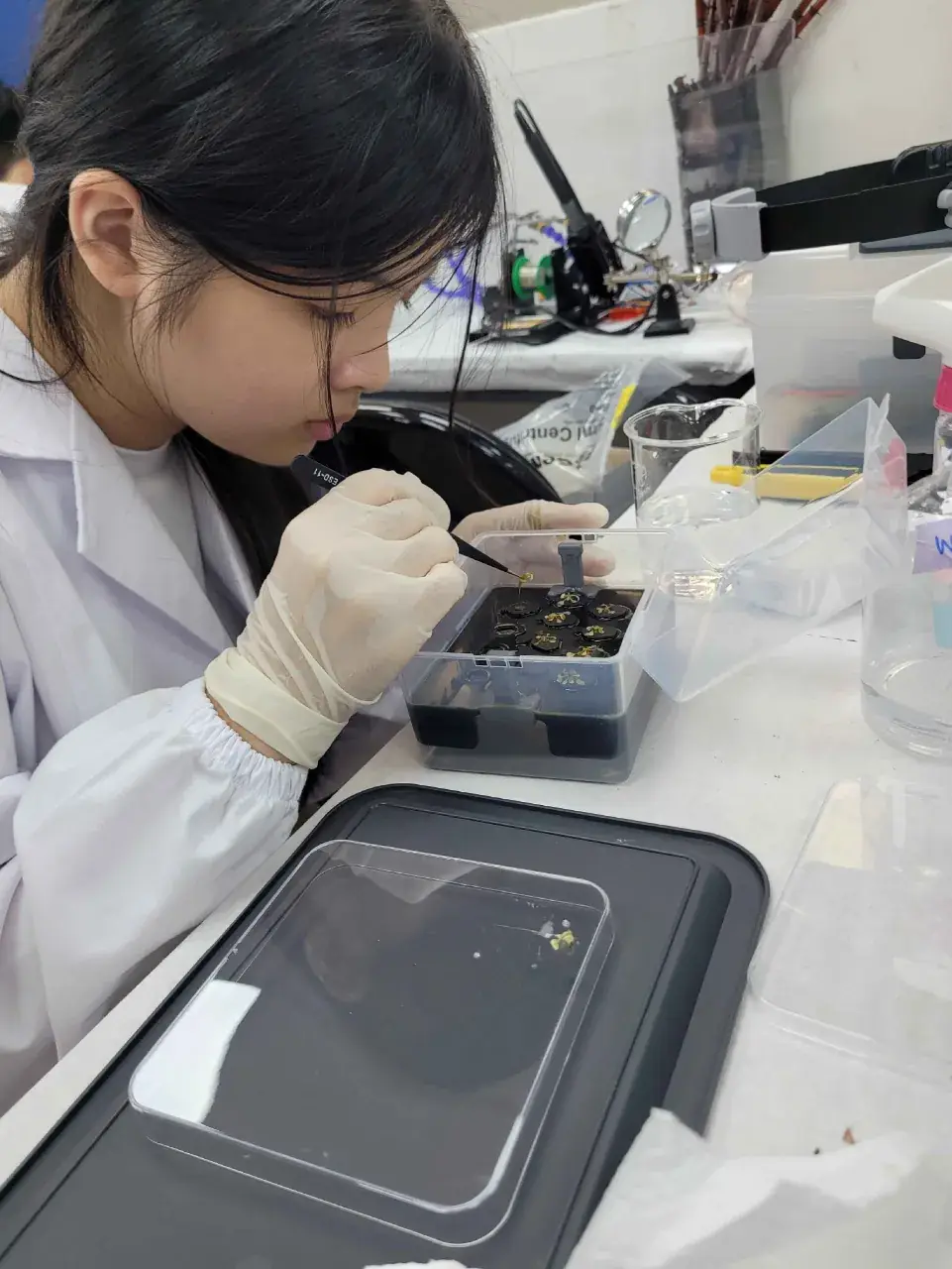
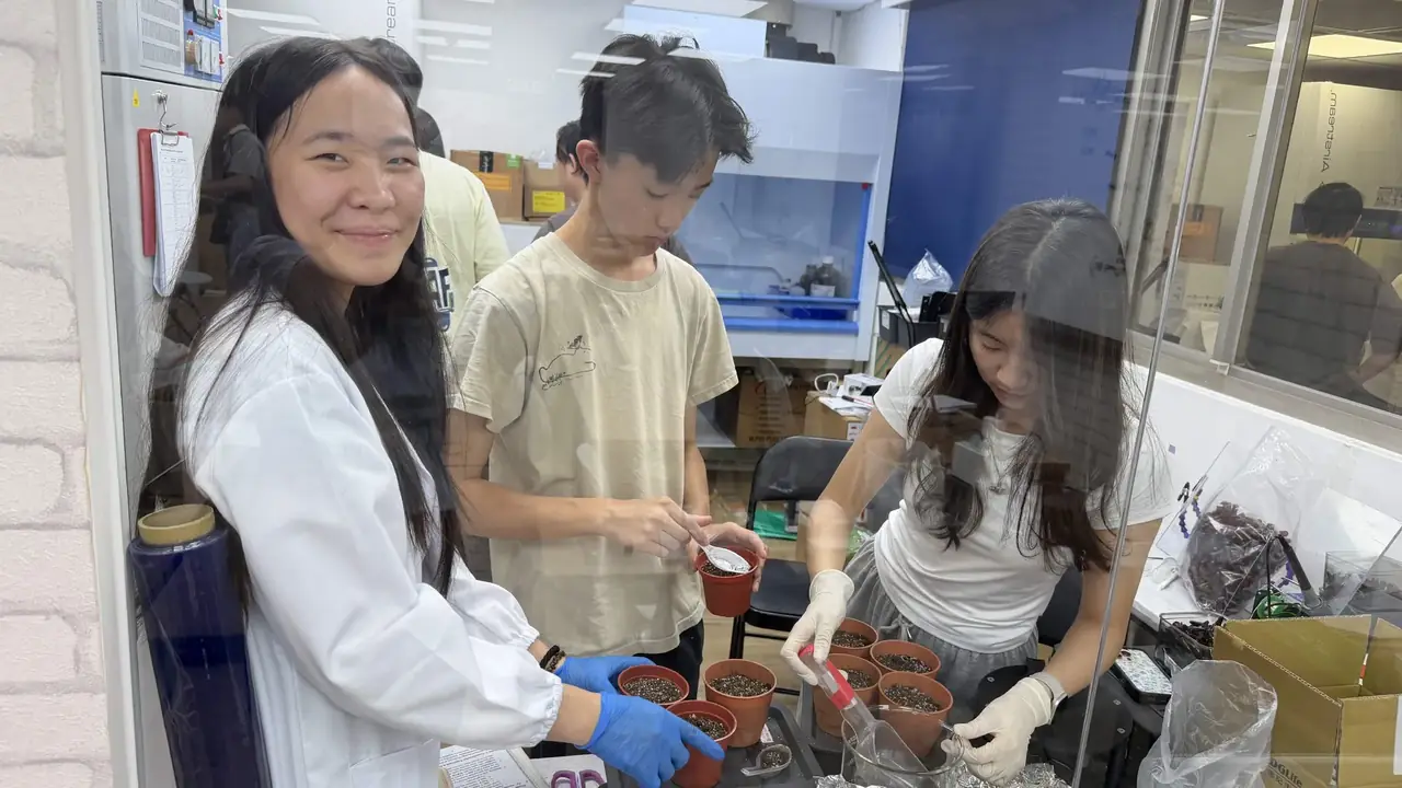
On agar at 75 mM, scored as fresh weight, pre-treatment is highest: 0.164 g against 0.144 g for co-treatment, about 14% more. In soil at 300 mM, scored as chlorophyll per gram, co-treatment is highest and pre-treatment has no effect; a commercial peptide at 100 mM also ranked co-treatment first. The soil run cannot settle the question. Its five tubes held 22 to 199 mg of tissue, each weighed once, and chlorophyll per gram tracks tissue weight at r = −0.85. The group that appears rescued is the smallest of the five, and read as total chlorophyll the same tubes rank co-treatment last.
An efficacy of 0.58, carried from Arabidopsis fresh weight on agar to rice grain yield, is withdrawn. Seedling growth and chlorophyll do not establish recovery of rice yield, the agar run reaches the ceiling of the calculation it came from, and the soil run cannot be read, so neither bounds the coefficient. M5 instead plots payback across efficacy, which identifies the yield benefit future rice trials would have to demonstrate.
From plate dose to capital per hectare
The preceding results combine here as one chain. A recorded volume over a known plate area is an application rate, and that rate scales to a hectare with no modelling step in between. The protocol specifies 10 cm round plates, so the area is 78.5 cm², and one plate treatment was three nozzle actuations delivering 1.67 mL in total. From there the titre converts litres to protectant, the weather record converts one application to a season, and the reactor's throughput converts a season to vessel volume and capital.
One step in that chain is weaker than the arithmetic around it. The titre and the applied volume come from different preparations: the activity is the 7 October supernatant assay, the volume is the spray protocol of Experiment #9, and the activity of the preparation applied to the plants was not measured. At the reported supernatant activity the scenario corresponds to 37.6 kU per hectare, an activity this model carries forward with no experiment behind it as an effective dose.
Two rows come with a caveat. The canopy correction is modelled from a leaf area index of 4.5 against 0.115 on a seedling plate and spans 1.68 to 3.52, so the 5,188 L is a scenario and not a validated rice dose. The experiment that produced 1.67 mL varied salt level and timing but not the applied amount, so 2,126 L/ha is the dose that worked and the smallest that works is unknown. A single plate with neat, 1:3, 1:10 and 1:30 arms would locate the minimum, and every row below it would move.
Payback and fleet utilisation
Ten units cost US$9,375. The stress index attributes US$138 per hectare per crop of loss on an ordinary Yunlin (雲林) paddy to the weather this protectant acts on. Under the current trigger only the second crop generates application windows, so one crop a year returns anything. Efficacy is the share of that loss the protectant recovers; no run of ours bounds it, so payback is plotted across the whole axis.
No point on that axis returns the capital on a useful horizon. At efficacy 1 the payback is 68 years, and five years would require an efficacy of 14, which exceeds the loss itself. Geospatial Analysis reaches a different figure from its own chlorophyll work: a net benefit of US$1,931 per hectare per crop, paying back in 4.9 years, which is 14 times the whole loss this index attributes to weather. The two rest on different stress definitions and different biological assumptions, so they are not yet two estimates of the same hectare. Section 5 sets out what would settle it.
The second constraint is utilisation. Only the second crop generates windows, and within it 17 of 25 seasons never cross the threshold. A qualifying season needs 9 passes, the median across the seasons that qualify on a provisional trigger and an assumed two-day protection window, at 5.4 days each, or 49 reactor-days inside a crop of about 120 days, so one ten-unit fleet covers 2.5 hectares and operates on 4.3% of the calendar.
Payback therefore depends on ownership. One fleet shared across the 2.5 hectares it can serve divides the capital accordingly: 27 years on this page's loss figure at efficacy 1, and 2.0 years on the Geospatial Analysis figure. On either benefit estimate, a reactor owned by a single farm is idle for most of its service life.
Links to the bench and to Geospatial Analysis
The measured rows of the ledger were produced by this team. The plate area and the applied volume come from the plant team's protocol, the titre and the light-plate readings from the measurement team's assays, and the throughput from the reactor team's batch cycle. Published constants, public records and the five assumptions of Section 3 fill the steps between them, and Section 2 records which is which.
The business team asked for three figures: the protectant one hectare of ordinary rice farmland requires, the gap between that and current reactor output, and the cost of closing it. The ledger was built to end on those three. All three carry the canopy correction, so they are scenario figures and not quotations.
| The question | The answer this model gives | Where in the model |
|---|---|---|
| How much protectant does one hectare need? | 37.6 kU per application and 339 kU in a season that fires, which at our secreted protein concentration is about 10 g and 92 g of enzyme | M4, the protectant group |
| How far is that from what we can make now? | One hectare needs 81 L of vessel running all season. The current spec is 10 × 20 L = 200 L, which covers 2.5 ha, about one Taiwanese farm. A 100-hectare association needs 8,106 L, a 41× scale-up | M4, the machine group, and M5 |
| What does that cost? | US$3,800 of capital per hectare at US$937.50 per 20-litre unit, before any refill, service or labour. For 100 hectares, US$379,992 | M4, the result line |
Geospatial Analysis answers a similar but distinct question. It derives units per hectare from soil class, which governs how far and how long the protectant remains where it is applied; this page derives units per hectare from reactor throughput, which governs whether enough can be made at all. A deployment has to satisfy both constraints, and the binding one will differ by township, so the two densities need reconciling before either is quoted as the number of machines a field requires.
The two pages also disagree on the benefit, by the factor of 14 set out in M5. Either this index misses most of what stress costs a field, or the chlorophyll-to-yield step in Geospatial Analysis is too generous. Three measurements would settle it: a yield endpoint in place of a chlorophyll one, a single stress definition across both pages, and agreement on whether a protected hectare returns once or twice a year. Until then this page quotes its own figure and marks where the other falls.
They agree on ownership by different routes. Geospatial Analysis puts capital per hectare at or above a full year of gross paddy revenue in every soil class; this page reaches the same place from utilisation, since a machine that stands idle for most of its service life cannot be bought by the farm it serves. With 99% of Taiwanese farmers working under two hectares, a shared asset held by a farmers' association is the only structure the arithmetic permits. Two costs a farmer pays are absent from this ledger: refill cartridges and hardware service life. The straw-return mechanism in the business plan acts on the first.
Conclusion
The model was built to size a dose and the binding result is the size of the equipment. Taiwan's harvest record supplies a stress index that carries 32% less county error than the no-weather trend in the second crop, and a frozen 2026 forecast is now being scored against the harvest. From there the chain is a few steps of arithmetic over one modelled correction: 37.6 kU of protectant per hectare, 81 litres of vessel to make it in a season, and US$3,800 of capital to buy them.
Two results constrain the system as specified. It takes 5.4 days to serve one hectare against a three-day forecast, so it has to operate on banked stock; and it covers 2.5 hectares while operating on 4.3% of the calendar, which puts individual ownership out of reach at the farm size 99% of Taiwanese farmers work. Geospatial Analysis reaches the same conclusion from soil and revenue rather than throughput.
Two results are unresolved. The secreted protectant loses activity with an apparent half-time of 0.7 to 1.5 hours, by two routes on the same material; neither measures storage lifetime, but activity on that timescale is too short for a system that has to hold stock. And the benefit a protected hectare returns is in dispute by a factor of 14 between this page and Geospatial Analysis. Neither gap closes with further modelling; both close at a bench, and Current limits states with what.
Equations
Six relations do the arithmetic. Two are the optogenetic transfer function and its inversion, two convert an assay reading to enzyme, and two convert enzyme to equipment and capital. Each is cited where it is not ours.
Steady-state output of PcpcG2 under CcaSR as a fraction of saturation, against green photon flux I. For B. subtilis, K1/2 = 4.66 ± 0.63 µmol m⁻² s⁻¹ and n = 1.88 ± 0.16 (Castillo-Hair et al., 2019). Used as published; every induction we have run was at one intensity, so we have not tested it.
Equation 1 inverted: the lamp setpoint that delivers a demand f from M1. The lamp ceiling of 20 µmol m⁻² s⁻¹ reaches 0.94 of maximum on this curve.
Michaelis–Menten, used to correct the DNPH reading to Vmax. At 43.0 mM substrate against Km = 3.4 mM the assay runs at 93% of Vmax (Hontzeas et al., 2004).
Active-site concentration from corrected activity, with kcat = 146 min⁻¹ for Pseudomonas putida UW4 (Hontzeas et al., 2004). At our titre this is 54 nM of sites, or 1.96 mg L⁻¹ of protein.
Litres of culture per hectare, from the volume applied over a known plate area scaled to 10⁸ cm², times the canopy correction C = 2.44. C is the only modelled term in this equation and spans 1.68 to 3.52. Two further figures in the ledger are not direct measurements either: the application schedule, which assumes a two-day protection window, and the reactor output R in Equation 6, which is derived from the batch cycle.
Vessel litres a hectare needs, from the dose, the passes a firing season takes, the reactor's output R in culture-litres per vessel-litre per day and the length of the crop; and the payback that capital K reaches at efficacy ε against an addressable loss L. Both are ours.
Current limits
Seven things this model cannot yet do. Efficacy is unbounded: no plant run of ours constrains how much of a salinity loss the protectant takes back, so every figure in dollars is drawn against efficacy and never at a value. The dose is one that worked, not the smallest that works, and no dilution series has been run. The canopy correction is modelled and spans 1.68 to 3.52, and every row of the ledger below it inherits that. The titre rests on a single supernatant assay below the quantitation limit, and the 28-hour endpoint that would check it cannot be distinguished from a stalled reaction. Shelf life has no direct measurement. What stands in for it is an apparent half-time of 0.7 to 1.5 hours by two routes, one of them an unreplicated pair read in live culture while the cells were still producing, so the figure bounds activity in the vessel and leaves the lifetime of a harvested preparation unmeasured. The banked-stock plan turns on whether it survives replication and on whether a concentrated, cooled or formulated preparation holds longer. The protection window is assumed at two days per pass, which is what fixes a firing season at nine passes. The release rule is counted from waterlogging while the payback is priced on salinity; making them agree means rebuilding the rule around salt-sensitive growth stages, which would need roughly fifteen applications in a 30-day window instead of nine, or 81 reactor-days inside 30, which the current fleet could not serve for even one hectare without banking well in advance.
References
Measurements made by this team are documented on Measurement, Plants and Notebook, and are cited in the tables above rather than listed here. Published sources follow APA 7.
- Agriculture and Food Agency, Ministry of Agriculture. (2026). Rice production statistics by county and crop season, 2001–2026 [Data set]. Republic of China (Taiwan).
- Arnon, D. I. (1949). Copper enzymes in isolated chloroplasts. Polyphenoloxidase in Beta vulgaris. Plant Physiology, 24(1), 1–15. https://doi.org/10.1104/pp.24.1.1
- Castillo-Hair, S. M., Baerman, E. A., Fujita, M., Igoshin, O. A., & Tabor, J. J. (2019). Optogenetic control of Bacillus subtilis gene expression. Nature Communications, 10, 3099. https://doi.org/10.1038/s41467-019-10906-6
- Central Weather Administration. (2026). Station observations and short-range forecasts [Data set]. Republic of China (Taiwan).
- Hersbach, H., Bell, B., Berrisford, P., Hirahara, S., Horányi, A., Muñoz-Sabater, J., Nicolas, J., Peubey, C., Radu, R., Schepers, D., Simmons, A., Soci, C., Abdalla, S., Abellan, X., Balsamo, G., Bechtold, P., Biavati, G., Bidlot, J., Bonavita, M., … Thépaut, J.-N. (2020). The ERA5 global reanalysis. Quarterly Journal of the Royal Meteorological Society, 146(730), 1999–2049. https://doi.org/10.1002/qj.3803
- Hontzeas, N., Zoidakis, J., Glick, B. R., & Abu-Omar, M. M. (2004). Expression and characterization of 1-aminocyclopropane-1-carboxylate deaminase from the rhizobacterium Pseudomonas putida UW4: A key enzyme in bacterial plant growth promotion. Biochimica et Biophysica Acta (BBA) — Proteins and Proteomics, 1703(1), 11–19. https://doi.org/10.1016/j.bbapap.2004.09.015